Convolution and Fourier Transform

The relationship between convolution and the Fourier transform.

Convolution

We will start with convolution. The Convolution operation takes two functions and produces a third function. It is defined as the integral of the product of the two functions after one is reversed and shifted. The convolution of two functions $f(t)$ and $g(t)$ is denoted by $f(t) * g(t)$ and is defined as:

$$(f * g)(t) = \int_{-\infty}^{\infty} f(\tau) g(t - \tau) d\tau$$

The minus sign accounts for the flipping, $t$ is the shifting variable needed to slide one function past the other, and $\tau$ is the dummy variable of integration.

The convolution of two functions is a third function that represents the amount of overlap between the two functions as one is shifted over the other. As we said before, the convolution operation is commutative, meaning that

$$f * g = g * f$$

It is also associative, meaning that

$$(f * g) * h = f * (g * h)$$

The convolution of a function with a delta function is the function itself, i.e. $f(t) * \delta(t) = f(t)$. The convolution of a function with a step function is the integral of the function, i.e.

$$f(t) * u(t) = \int_{-\infty}^{t} f(\tau) d\tau$$

Convolution Theorem

The convolution theorem states that the Fourier transform of the convolution of two functions is equal to the product of their Fourier transforms. Mathematically, the convolution theorem is stated as:

$$\mathcal{F}\{f * g\} = \mathcal{F}\{f\} \cdot \mathcal{F}\{g\}$$

where $\mathcal{F}\{f\}$ and $\mathcal{F}\{g\}$ are the Fourier transforms of $f(t)$ and $g(t)$, respectively. The convolution theorem is very useful in signal processing and communication systems. It allows us to perform convolution in the time domain by simply multiplying the Fourier transforms of the two functions and then taking the inverse Fourier transform of the result. This is much easier than performing the convolution directly in the time domain.

Proof of the Convolution Theorem

The proof of the convolution theorem is quite simple. We start with the definition of the Fourier transform of the convolution of two functions:

$$\mathcal{F}\{f * g\} = \int_{-\infty}^{\infty} (f * g)(t) e^{-j\omega t} dt$$

Using the definition of the convolution, we can write the above equation as:

$$\mathcal{F}\{f * g\} = \int_{-\infty}^{\infty} \left[ \int_{-\infty}^{\infty} f(\tau) g(t - \tau) d\tau \right] e^{-j\omega t} dt$$

We can interchange the order of integration (I think its called Fubini's Theorem, whatever close enough) and write the above equation as:

$$\mathcal{F}\{f * g\} = \int_{-\infty}^{\infty} f(\tau) \left[ \int_{-\infty}^{\infty} g(t - \tau) e^{-j\omega t} dt \right] d\tau$$

The integral inside the square brackets is the Fourier transform of $g(t - \tau)$, which is $G(\omega) e^{-j\omega \tau}$. This leverages the shift property of the Fourier transform, specifically $\mathcal{F}\{g(t - \tau)\} = G(\omega) e^{-j\omega \tau}$. This is how the time-domain shift becomes a phase shift in the frequency domain.

Substituting this into the above equation, we get:

$$\mathcal{F}\{f * g\} = \int_{-\infty}^{\infty} f(\tau) G(\omega) e^{-j\omega \tau} d\tau$$

This is the product of the Fourier transform of $f(t)$ and $g(t)$, i.e. $\mathcal{F}\{f\} \cdot \mathcal{F}\{g\}$. More specifically,

$$\begin{align*} \mathcal{F}\{f * g\} &= G(\omega) \int_{-\infty}^{\infty} f(\tau) e^{-j\omega \tau} d\tau \\ &= \mathcal{F}\{f\} \cdot \mathcal{F}\{g\} \end{align*}$$

So, we have $G(\omega)F(\omega)$, which is the product of the Fourier transforms of $f(t)$ and $g(t)$. I hope this completes the proof of the convolution theorem.

Deconvolution

Linear, Position-Invariant Degradations

Let's quickly discuss the properties of the linear operator. A linear operator is a mapping between two vector spaces that preserves the vector space structure. In the context of image processing, a linear operator is a transformation that satisfies the following two properties:

1. Additivity: $L(a \cdot f + b \cdot g) = a \cdot L(f) + b \cdot L(g)$

2. Homogeneity: $L(c \cdot f) = c \cdot L(f)$

where $L$ is the linear operator, $f$ and $g$ are the input functions, and $a$, $b$, and $c$ are constants. You have seen this a million times and can prove these with your eyes closed by now.

A position-invariant degradation is a type of linear operator that does not depend on the position of the input function. In other words, the output of the operator at a given position is only determined by the input at that position. Maybe you heard this property known as shift-invariance or translation-invariance.

In optics, the impulse becomes a point of light and the response of the system is the point spread function (PSF). The PSF is the response of the system to a point of light. The PSF is a measure of the blurring effect of the system. The PSF is a position-invariant degradation because it does not depend on the position of the input function.

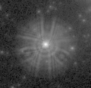
The point spread function of Hubble Space Telescope's WFPC camera before corrections were applied to its optical system¹.

Some example point spread functions are the Gaussian PSF, the Airy disk, and the Lorentzian PSF. They are defined as follows:

• Gaussian PSF: $h(x, y) = \frac{1}{2\pi\sigma^2} e^{-\frac{x^2 + y^2}{2\sigma^2}}$

• Airy Disk: $h(x, y) = \frac{J_1(\pi r/\lambda)}{\pi r/\lambda}$

• Lorentzian PSF: $h(x, y) = \frac{1}{\pi} \frac{\gamma}{x^2 + y^2 + \gamma^2}$

where $h(x, y)$ is the PSF, $x$ and $y$ are the spatial coordinates, $\sigma$ is the standard deviation of the Gaussian, $J_1$ is the Bessel function of the first kind, $r$ is the radius of the Airy disk, $\lambda$ is the wavelength of light, and $\gamma$ is the half-width at half-maximum of the Lorentzian.

You can apply these to images in Python using the following code:

import numpy as np
import matplotlib.pyplot as plt
from scipy.signal import convolve2d

# Create a Gaussian PSF
def gaussian_psf(x, y, sigma):
    return 1 / (2 * np.pi * sigma**2) * np.exp(-(x**2 + y**2) / (2 * sigma**2))

# Create a grid of spatial coordinates
x = np.linspace(-5, 5, 100)
y = np.linspace(-5, 5, 100)
X, Y = np.meshgrid(x, y)

# Compute the Gaussian PSF
sigma = 1
psf = gaussian_psf(X, Y, sigma)

# Display the Gaussian PSF
plt.imshow(psf, cmap='gray')
plt.axis('off')

# Convolve the PSF with an image
image = np.random.rand(100, 100)
blurred_image = convolve2d(image, psf, mode='same')

# Display the original and blurred images
plt.figure()
plt.subplot(1, 2, 1)
plt.imshow(image, cmap='gray')
plt.axis('off')
plt.title('Original Image')
plt.subplot(1, 2, 2)
plt.imshow(blurred_image, cmap='gray')
plt.axis('off')
plt.title('Blurred Image')
plt.show()

The code creates a Gaussian PSF and convolves it with a random image to produce a blurred image. You can experiment with different PSFs and images to see the effects of different types of blurring.

Intro to Deconvolution Operations

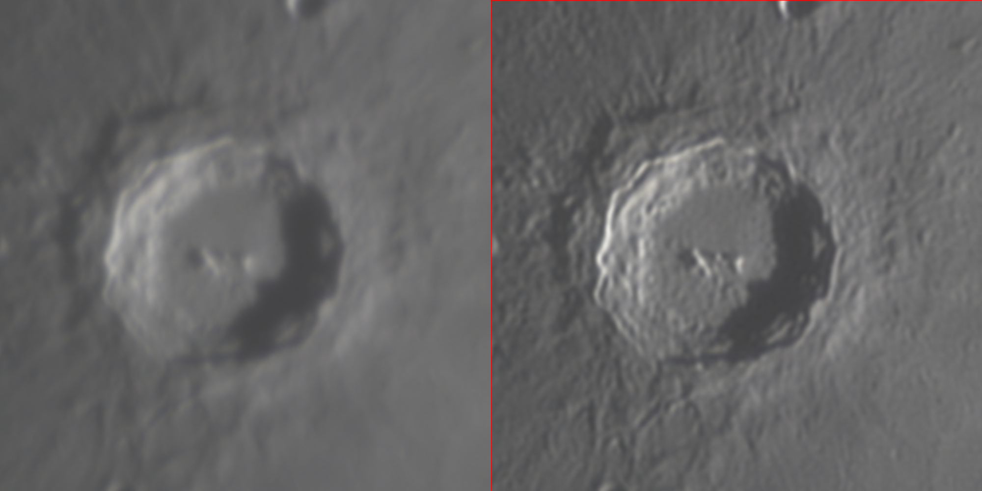
Before and after deconvolution of an image of the lunar crater Copernicus using the Richardson-Lucy algorithm. The image on the left is the original image, and the image on the right is the deconvolved image².

Deconvolution, within the realm of signal processing, is a mathematical operation aimed at reversing the effects of convolution on a signal. It is analogous to solving for an unknown in a division operation when the product and one multiplicand are known. Similarly, given a convolved signal $n$, and the impulse response $m$ of the system, deconvolution seeks to recover the original signal $x$, such that $x = \frac{n}{m}$ in the context of convolution operations.

In practical terms, deconvolution is typically performed in the Fourier domain. This involves dividing the Fourier transform of the convolved signal by the Fourier transform of the system's impulse response, each represented as complex numbers (e.g., $a + ib$ and $c + id$, respectively). The division follows the rules for complex numbers, and the result is then inverse-transformed to retrieve the original signal in the time or spatial domain. This process leverages the Fourier transform's capability to convert convolution operations in the time or spatial domain into multiplication operations in the frequency domain, thus simplifying the deconvolution to a division operation.

It is crucial to distinguish between the two contexts in which "deconvolution" is used. One refers to the Fourier deconvolution process, where the convolution's broadening function is known but the original signal's exact form is not. The other context involves iterative least-squares curve fitting, where the exact form of the peak is known, but the broadening parameters are not. Despite both being termed "deconvolution," they serve distinct purposes and should not be confused.

Fourier deconvolution holds significant practical value in signal processing for its ability to computationally reverse convolution effects that occur in physical systems. This can include correcting signal distortions introduced by electrical filters or compensating for the finite resolution of measuring instruments like spectrometers. By applying a known impulse (or "delta") function to the system and measuring the output, one can obtain the necessary data for deconvolution, thereby elucidating the characteristics of the convolution process itself or recovering the undistorted original signal³.

Technical Overview of Deconvolution

At its core, deconvolution seeks to estimate the original signal $f(t)$ from the observed signal $g(t)$, which results from the convolution of $f(t)$ with a known impulse response $h(t)$ of the system, alongside potential additive noise. Mathematically, the relationship can be represented as:

$$g(t) = (f \ast h)(t) + n(t)$$

where $\ast$ denotes the convolution operation and $n(t)$ represents noise. The challenge of deconvolution lies in accurately inverting this relationship to solve for $f(t)$, especially in the presence of noise.

Richardson-Lucy Deconvolution

The Richardson-Lucy algorithm is an iterative method particularly popular in astronomical imaging and microscopy, where the point spread function (PSF), corresponding to $h(t)$ in our notation, is known. This algorithm is grounded in Bayesian inference, aiming to maximize the likelihood of observing $g(t)$ given $f(t)$, under Poisson noise considerations.

Algorithmic Framework

The Richardson-Lucy algorithm iteratively refines the estimate of $f(t)$ through the following update rule:

$$f_{n+1}(t) = f_n(t) \cdot \frac{g(t)}{(f_n \ast h)(t)} \ast h(-t)$$

where $f_{n}(t)$ is the estimate of the original signal at the $n^{th}$ iteration, and $h(-t)$ is the impulse response flipped in time. This process incrementally improves $f(t)$'s estimate by comparing the convolved estimate with the observed signal $g(t)$, adjusting based on the discrepancy.

Python Implementation

The Richardson-Lucy algorithm can be implemented in Python using the following code:

import numpy as np
from scipy.signal import fftconvolve

def richardson_lucy(g, h, iterations):
    f = np.ones_like(g)
    h_flipped = np.flip(h)
    for _ in range(iterations):
        f = f * fftconvolve(g / (fftconvolve(f, h, mode='same') + 1e-10), h_flipped, mode='same')
    return f

# Example usage
g = np.random.poisson(100, size=100)
h = np.exp(-np.linspace(-5, 5, 100)**2)
f = richardson_lucy(g, h, iterations=100)

In this code, g is the observed signal, h is the known impulse response, and iterations is the number of iterations for the Richardson-Lucy algorithm. The richardson_lucy function iteratively updates the estimate of the original signal f using the Richardson-Lucy update rule. The fftconvolve function is used for fast convolution in the frequency domain.

Fergus's Method

Fergus et al. introduced a method focusing on removing camera shake from photographs, an application where the PSF ($h(t)$) is typically unknown and must be estimated alongside the original image $f(t)$. This approach combines machine learning techniques with deconvolution, using a prior knowledge of typical camera PSFs and natural image statistics.

Algorithmic Insights

The method by Fergus and colleagues employs a two-step iterative process:

1. PSF Estimation: Given an initial estimate of $f(t)$, the algorithm updates the PSF estimate by maximizing the likelihood of $g(t)$ given $f(t)$ and the current PSF estimate.
2. Signal Recovery: With the updated PSF, the algorithm refines $f(t)$'s estimate using techniques akin to Richardson-Lucy deconvolution or other suitable deconvolution strategies, incorporating image priors to regularize the solution.

This method stands out by addressing the blind deconvolution problem, where both the original signal and the system's impulse response are unknown, showcasing the interplay between signal processing techniques and machine learning in modern image restoration tasks.

Pseudocode

The implementation of Fergus's method in Python involves a more complex pipeline, combining machine learning models (think sklearn) for PSF estimation with deconvolution algorithms for signal recovery. The process typically involves training a model to estimate the PSF from the observed image and then using the estimated PSF in a deconvolution algorithm to recover the original signal. Due to the complexity of this approach, a detailed implementation is beyond the scope of this overview.

Nonetheless, I will provide a VERY high level of the steps involved in the process:

1. Load the blurred image
   - Input: Path to the blurred image
   - Output: Blurred image matrix

2. Simulate or estimate the initial Point Spread Function (PSF)
   - Method: Assume a horizontal motion blur (for simulation)
   - Output: Initial PSF matrix

3. Refine PSF estimate using Machine Learning
   - Extract features from the blurred image (e.g., pixel values, gradients)
   - Set up a Machine Learning model (e.g., Polynomial Regression)
   - Train the model using the blurred image features and the initial PSF as targets
   - Predict a refined PSF using the trained model

4. Perform deconvolution using the refined PSF
   - Method: Apply an inverse filter or a more sophisticated deconvolution algorithm
     like Richardson-Lucy or Wiener filter, using the refined PSF
   - Input: Blurred image and refined PSF
   - Output: Deconvolved (restored) image

5. Display or save the deconvolved image
   - Show the original blurred image, the initial PSF, the refined PSF, and the deconvolved image

Explanation of Steps

• Step 1: This is where you load the image that has been blurred, either due to motion, out-of-focus capture, or other reasons. This image is what you'll be working to deconvolve.

• Step 2: An initial guess or estimate of the PSF is necessary because it represents how the image got blurred. In practice, this might come from knowledge about the camera or the type of motion that caused the blur.

• Step 3: Refining the PSF is crucial for accurate deconvolution. This step involves using machine learning to adjust the initial PSF based on the observed blurred image. The idea is to learn a PSF that, when used to blur a sharp image, would result in the observed blurred image.

• Step 4: With the refined PSF, you can now attempt to reverse the blurring process. This involves computational techniques that aim to invert the effect of convolution (blurring) to restore the original sharp image.

• Step 5: Finally, comparing the deconvolved image with the original blurred image and the PSFs can provide insight into the effectiveness of the deconvolution process and the accuracy of the PSF refinement.

Yes, deconvolution is hard

Deconvolution is a powerful, albeit challenging, operation in signal processing that requires careful consideration of the system's characteristics and the nature of the noise. The Richardson-Lucy algorithm and Fergus's method illustrate two approaches tailored to specific applications, emphasizing the importance of accurate PSF modeling and the benefits of incorporating prior knowledge for effective signal restoration. These methodologies underscore the broader theme in signal processing: the extraction of meaningful information from distorted observations. Ahh yes, the complexities of real-world signals.

---

Paper | Coded Exposure Photography: Motion Deblurring using Fluttered Shutter

Paper to Read

Please read the following paper "Coded Exposure Photography: Motion Deblurring Using Fluttered Shutter" by Ramesh Raskar et al.⁴ to understand the application of deconvolution in image processing.

In the realm of image processing, capturing clear images of moving objects remains a significant challenge due to motion blur. This blur occurs when the camera's shutter is open long enough for the movement of the subject or the camera itself to be recorded as a blur. Traditional photography techniques often struggle to balance the need for sufficient light with the desire to freeze motion, especially in low-light conditions.

The Problem: Motion blur in photographs

The primary issue addressed by the paper "Coded Exposure Photography: Motion Deblurring Using Fluttered Shutter" by Ramesh Raskar et al. is motion blur in photographs. Motion blur significantly degrades image quality, particularly in low-light conditions or when capturing fast-moving subjects. Traditional methods to reduce motion blur, such as shortening the exposure time, increasing lighting, or using flash, are not always practical or effective and can introduce other trade-offs like noise or loss of ambient scene details.

The Solution: Coded exposure photography using a fluttered shutter

The authors propose an innovative solution to the motion blur problem: coded exposure photography using a fluttered shutter. This technique involves modulating the camera's exposure over time in a coded pattern, allowing more light in while still capturing sharp images of moving objects. The key innovation lies in the ability to deblur the images post-capture, using the known exposure pattern to reverse the motion blur in a way that traditional photography cannot.

Key Contributions Section

The authors broke down the motion deblurring problem into three parts: capture-time decision for motion encoding, PSF estimation and image deconvolution. The key novelty of their methods stem from modifying the capture-time temporal integration to minimize the loss of high spatial frequencies of blurred objects.

• Computed a near-optimal binary coded sequence for modulating the exposure and analyze the invertibility of the process,
• Presented techniques to decode images of partially-occluded background and foreground objects,
• Showed how to handle extremely large degrees of blur.

Their Method

The method involves the following key steps:

1. Coded Shutter: Instead of a constant open/close shutter action, the shutter rapidly opens and closes in a predefined pattern during the exposure time. This pattern is designed to encode motion information into the captured image.

2. Motion Deblurring: The captured image, which contains motion-blurred information encoded through the fluttered shutter, is processed using an algorithm that understands the coded pattern. This algorithm mathematically reverses the motion blur, reconstructing a sharp image of the moving subject.

3. Algorithmic Reconstruction: The deblurring process utilizes the known coded exposure pattern and applies a deconvolution algorithm. This step is crucial for decoding the motion information and restoring image clarity.

Mathematical Model

The authors developed a mathematical model to describe the motion blur as a convolution of the scene motion with the camera's exposure function. This model allowed them to design a coded exposure pattern that would minimize the loss of high spatial frequencies of blurred objects. They also developed an algorithm to decode the motion information and reconstruct the sharp image.

Relevance to Image Processing Class

This paper's approach to motion deblurring is highly relevant to our image processing class for several reasons:

• Innovative Use of Image Processing Techniques: It demonstrates a creative application of deconvolution and algorithmic image reconstruction, key topics in our course.
• Understanding of Motion Blur: It offers a practical understanding of motion blur as a convolution of the scene motion with the camera's exposure function, aligning with our studies on convolution and filtering.
• Algorithmic Problem Solving: The method showcases how algorithms can solve real-world problems in image processing, emphasizing the importance of mathematical models in developing practical solutions.
• Exposure to Cutting-edge Research: Exploring this paper gives students insight into how current research addresses complex challenges in photography and image processing, encouraging innovation and application of course concepts to novel problems.

This is a very quick overview and I did not go over all the details of the paper here. I encourage you to read the paper to understand the full scope of the problem and especially the parts I discussed here on the authors' approach to solving the problem.

Footnotes

1. https://en.wikipedia.org/wiki/Point_spread_function ↩

2. https://en.wikipedia.org/wiki/Deconvolution ↩

3. O'Haver, T. "Intro to Signal Processing - Deconvolution". University of Maryland at College Park. http://www.wam.umd.edu/~toh/spectrum/Deconvolution.html ↩

4. Ramesh Raskar, Amit Agrawal, and Jack Tumblin. 2006. Coded exposure photography: motion deblurring using fluttered shutter. In ACM SIGGRAPH 2006 Papers (SIGGRAPH '06). Association for Computing Machinery, New York, NY, USA, 795–804. https://doi.org/10.1145/1179352.1141957 ↩